College Basketball Player Value Model: Box Plus-Minus for NCAA Men's Players

Box plus-minus (BPM) estimates how many points per 100 possessions a player adds over an average player, using only what appears in the box score. It cannot see a great screen or a help rotation, but it is stable in small samples, which on/off measures are not. load_mbb_player_value() returns offensive, defensive and total box plus-minus for every men’s college player-season. This article explains the model, how reliable it is, and how to filter it sensibly.

The official model card is player_value.md in the hoopR-mbb-data repository. Numbers below are computed here from the published release unless labeled “as reported in the model card”.

What does the dataset contain?

Column	Meaning
`box_obpm`	Offensive box plus-minus: points per 100 possessions added on offense.
`box_dbpm`	Defensive box plus-minus.
`box_bpm`	`box_obpm + box_dbpm`.
`min`	Minutes played.
`qualified`	`TRUE` when `min >= 300`, the floor at which the spread of BPM stops shrinking (see below).
`player_id`, `player`, `team_id`, `season`	Identifiers; `team_id` is the ESPN team id.

How is BPM computed?

As described in the model card:

Per-100 box features. For each player, sixteen rates from the box score: usage, true shooting and effective FG%, assist, turnover, offensive and defensive rebound, block and steal percentages, free-throw rate, shot shares at the rim, mid-range and three, and points, rebounds and assists per 100 possessions.
Standardize and score. Each feature is standardized (z-scores clipped at 4) and scored through ridge-regression coefficients fit at the team level, separately for offense and defense.
Team constraint. A uniform adjustment per team makes the minutes-weighted sum of its players’ scores equal the team’s adjusted efficiency margin, so BPM adds up to team strength. (The team ratings are the subject of the team ratings article.)

The model is compute-on-demand: every publish recomputes BPM from the current season data, and the fitted coefficients ship beside the release as mbb_player_value_coefficients.json.

coef_url <- paste0(
  "https://github.com/sportsdataverse/sportsdataverse-data/releases/download/",
  "mbb_player_value/mbb_player_value_coefficients.json"
)
co <- tryCatch(jsonlite::fromJSON(coef_url), error = function(e) NULL)

if (!is.null(co)) {
  cat("method:", co$method, "| train seasons:", paste(co$train_seasons, collapse = ", "),
      "| ridge lambda offense/defense:", co$lambda_o, "/", co$lambda_d,
      "| z clip:", co$z_clip, "| fit floor (minutes):", co$min_minutes, "\n")
  # coefficient vectors are [intercept, slopes...] over feature_cols
  tibble::tibble(
    feature = co$feature_cols,
    obpm_slope = co$obpm_coef[-1],
    dbpm_slope = co$dbpm_coef[-1]
  ) |>
    dplyr::arrange(dplyr::desc(abs(obpm_slope) + abs(dbpm_slope))) |>
    dplyr::mutate(dplyr::across(-feature, \(x) round(x, 3)))
}
#> method: team_constrained_game_z | train seasons: 2025, 2026 | ridge lambda offense/defense: 300 / 100 | z clip: 4 | fit floor (minutes): 150
#> # A tibble: 16 × 3
#>    feature     obpm_slope dbpm_slope
#>    <chr>            <dbl>      <dbl>
#>  1 pts_per100       2.35      -2.02 
#>  2 usage           -2.40       1.64 
#>  3 ast_per100       1.59      -1.23 
#>  4 ts_pct           1.89       0.304
#>  5 reb_per100       1.2        0.337
#>  6 tov_pct         -1.25       0.174
#>  7 rim_share       -0.752      0.56 
#>  8 blk_pct          0.691     -0.531
#>  9 ftr              0.527     -0.538
#> 10 three_share      0.455     -0.353
#> 11 mid_share        0.442     -0.301
#> 12 efg_pct         -0.564      0.103
#> 13 ast_pct         -0.051      0.458
#> 14 oreb_pct         0.325     -0.106
#> 15 dreb_pct        -0.325      0.106
#> 16 stl_pct          0.018      0.28

Each slope is the change in BPM for a one-standard-deviation change in that feature, so slopes are directly comparable. Usage and efficiency carry opposite signs on offense: volume is penalized until it is efficient. Intercepts are absorbed by the team adjustment.

Loading the ratings

library(hoopR)
library(dplyr)
library(ggplot2)

pv <- load_mbb_player_value(seasons = 2020:2026)

pv |>
  group_by(season) |>
  summarise(players = n(), total_minutes = round(sum(min)),
            qualified_players = sum(qualified, na.rm = TRUE))
#> # A tibble: 7 × 4
#>   season players total_minutes qualified_players
#>    <int>   <int>         <dbl>             <int>
#> 1   2020    8750       2324478              2915
#> 2   2021    6837       1725931              2477
#> 3   2022    9359       2404751              2971
#> 4   2023    9717       2509140              3024
#> 5   2024    9838       2516161              3056
#> 6   2025    9795       2535605              3065
#> 7   2026    9990       2539283              3114

Why the 300-minute qualified flag?

The file keeps every player, including those with a few minutes. The most extreme BPM values belong to players with tiny samples. The spread of BPM by minutes played shows where it settles:

pv |>
  mutate(minutes_bin = cut(min, c(0, 50, 100, 200, 300, 400, 600, 800, 1000, Inf),
                           right = FALSE, dig.lab = 4)) |>
  group_by(minutes_bin) |>
  summarise(players = n(), sd_box_bpm = round(sd(box_bpm), 2),
            abs_bpm_p99 = round(quantile(abs(box_bpm), 0.99), 2))
#> # A tibble: 9 × 4
#>   minutes_bin players sd_box_bpm abs_bpm_p99
#>   <fct>         <int>      <dbl>       <dbl>
#> 1 [0,50)        33249       6.89       18.4 
#> 2 [50,100)       4227       5.19       13.9 
#> 3 [100,200)      3498       4.84       13.2 
#> 4 [200,300)      2690       4.43       12.2 
#> 5 [300,400)      2653       4.03       10.1 
#> 6 [400,600)      5093       3.97       10.2 
#> 7 [600,800)      5321       3.76        9.89
#> 8 [800,1000)     4799       3.69        9.91
#> 9 [1000,Inf)     2756       3.48        9.33

pv |>
  filter(season == 2026) |>
  ggplot(aes(min, box_bpm)) +
  geom_point(alpha = 0.15, size = 0.7, colour = "#2C3D50") +
  geom_vline(xintercept = 300, colour = "#B2182B", linetype = "dashed") +
  labs(
    title = "Small samples produce the extreme BPMs",
    subtitle = "2025-26; dashed line at the 300-minute qualified floor",
    x = "Minutes played", y = "Box plus-minus (points per 100 possessions)",
    caption = "Data: hoopR::load_mbb_player_value()"
  ) +
  theme_minimal()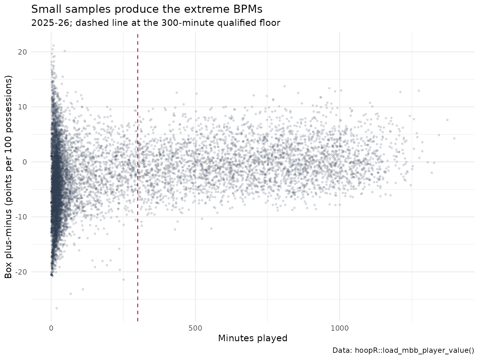

Scatter plot of box plus-minus against minutes played for 2025-26 men's college basketball players, showing a funnel that narrows as minutes increase, with a vertical line at 300 minutes.

As reported in the model card, the floor was set where the standard deviation of BPM first comes within 10% of its plateau at 600 to 800 minutes, using the published 2014-2026 seasons. Filter with qualified instead of re-deriving a threshold. (The model’s own 150-minute fit floor only governs the team-sum weights; the two floors answer different questions.)

How reliable is it?

A box-score model’s main virtue is persistence: a returning player’s BPM should carry over from season to season even with college basketball’s roster churn.

q <- pv |> filter(qualified) |> distinct(player_id, season, .keep_all = TRUE)

yoy <- q |>
  select(player_id, season, box_bpm) |>
  inner_join(q |> transmute(player_id, season = season - 1, box_bpm_next = box_bpm),
             by = c("player_id", "season"))

q26 <- filter(q, season == 2026)

c(
  yoy_pairs = nrow(yoy),
  yoy_r = round(cor(yoy$box_bpm, yoy$box_bpm_next), 3),
  qualified_2026 = nrow(q26),
  cor_obpm_dbpm_2026 = round(cor(q26$box_obpm, q26$box_dbpm), 3)
)
#>          yoy_pairs              yoy_r     qualified_2026 cor_obpm_dbpm_2026 
#>          10106.000              0.751           3114.000              0.151

Year-over-year correlation for qualified players is high (the model card reports 0.767 over all published seasons), and the offensive and defensive components are only weakly correlated, so they carry different information.

Who rated highest in 2025-26?

team_names <- load_mbb_team_box(seasons = 2026) |>
  distinct(team_id = as.character(team_id), team = team_display_name)

q26 |>
  mutate(team_id = as.character(team_id)) |>
  left_join(team_names, by = "team_id") |>
  arrange(desc(box_bpm)) |>
  select(player, team, min, box_obpm, box_dbpm, box_bpm) |>
  mutate(min = round(min), across(starts_with("box"), \(x) round(x, 2))) |>
  head(15)
#> # A tibble: 15 × 6
#>    player             team                   min box_obpm box_dbpm box_bpm
#>    <chr>              <chr>                <dbl>    <dbl>    <dbl>   <dbl>
#>  1 Tobe Awaka         Arizona Wildcats       809     7.33     6.4     13.7
#>  2 Oscar Cluff        Purdue Boilermakers    964    10.1      3.29    13.4
#>  3 Morez Johnson Jr.  Michigan Wolverines   1005     7.16     5.82    13.0
#>  4 Cameron Boozer     Duke Blue Devils      1274    10.4      2.49    12.9
#>  5 Motiejus Krivas    Arizona Wildcats       984     8.77     4.05    12.8
#>  6 Yaxel Lendeborg    Michigan Wolverines   1210     9.59     3.12    12.7
#>  7 Kalifa Sakho       Houston Cougars        435     5.48     7.1     12.6
#>  8 Rueben Chinyelu    Florida Gators         856     5.98     6.53    12.5
#>  9 Micah Handlogten   Florida Gators         504     4.38     8.01    12.4
#> 10 Patrick Ngongba II Duke Blue Devils       702     8.35     3.73    12.1
#> 11 Keba Keita         BYU Cougars            747     7.38     4.58    12.0
#> 12 Ernest Udeh Jr.    Miami Hurricanes       933     6.64     5.09    11.7
#> 13 Aday Mara          Michigan Wolverines    935     7.74     3.98    11.7
#> 14 Maliq Brown        Duke Blue Devils       769     2.67     8.72    11.4
#> 15 Sananda Fru        Louisville Cardinals   770     7.11     4.11    11.2

BPM versus RAPM

Box plus-minus and on/off RAPM (college RAPM model) deliberately measure different things. BPM sees only the box score, so it is stable in small samples but blind to screening, defensive attention and spacing. RAPM sees everything that changes the score but is noisy for low-minute players. Use them as cross-references. The natural hybrid, a RAPM that shrinks toward a box-score prior, is what the NBA player impact suite does with its adj-RAPM column.

Limitations

Box-score blind spots, as above; defense is especially hard to see in a box score.
Context. Rates depend on role and teammates; a high-usage scorer on a weak team and a role player on a strong one are scored on the same coefficients.
Team constraint. Because players sum to the team’s adjusted margin, a player on a strong team inherits some of that strength.
Low-minute rows. They are published, flagged qualified = FALSE. Filter them before ranking.

Where to go next

College basketball RAPM model and team ratings model.
NBA player impact model for SPM, BPM and adj-RAPM in the NBA.
Basketball advanced metrics for the rates (usage, TS%, eFG%) BPM is built from.
Reference: load_mbb_player_value() in the Model Dataset Loaders section.

Saiem Gilani