NBA and College Basketball Shot Charts in R with hoopR, sportyR and sdvplotR

A shot chart puts every field-goal attempt where it happened. It is the most direct picture of how a player or team scores, and with hoopR’s shot loaders and a court drawn by sportyR it takes a few lines of ggplot2. This article covers make/miss charts, hexbin and density maps, shot zones and field-goal percentage (FG%) by zone, for the NBA and men’s college basketball. Every chart is computed from one season of release data, filtered to one player where possible to keep it fast.

New to hoopR? Read Getting Started with hoopR first.

Packages

library(hoopR)
library(dplyr)
library(ggplot2)
library(sportyR)   # install.packages("sportyR")

season <- 2026     # the 2025-26 season

sdvplotR is optional. It adds sdv_court_coords(), which converts NBA Stats shot locations to sportyR’s court frame, and sdv_surface(), which paints a sportyR court in a team’s colors:

pak::pak("sportsdataverse/sdvplotR")

Which shot data does hoopR have, and in which coordinate frame?

Shot locations come in different frames, and mixing them up is the most common shot-chart bug.

Loader	Source	Location columns	Frame
`load_nba_shots()`	ESPN NBA play-by-play	`coordinate_x`, `coordinate_y`	Feet from center court; each team’s shots at the basket it attacks. Plot directly.
`load_mbb_shots()`	ESPN men’s college play-by-play	`coordinate_x`, `coordinate_y`	Same as above. A few rows hold placeholder values far off the court.
`load_nba_stats_shots()`	NBA Stats API	`x_legacy`, `y_legacy`	Tenths of a foot, origin at the hoop. Convert with `sdvplotR::sdv_court_coords()`.
`load_ncaa_mbb_shots()`	stats.ncaa.org engine	see its reference page	NCAA shot events from the play-by-play engine.

sportyR draws courts with the origin at center court, in feet: x runs along the court from -47 to 47 and y across it from -25 to 25. The left basket is at x = -41.75. geom_basketball("nba", display_range = "defense") draws the left half.

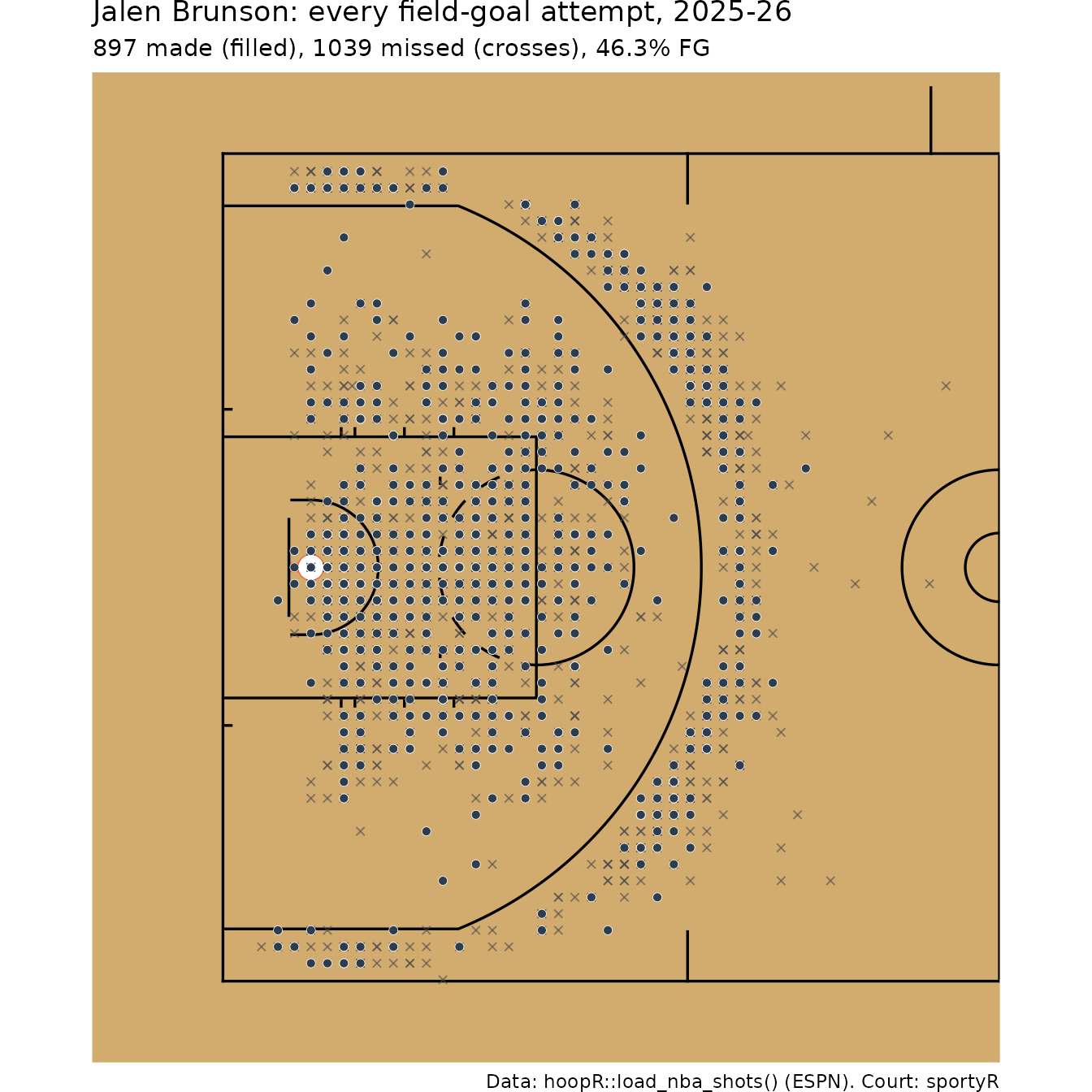
A make/miss chart for an NBA player

load_nba_shots() holds every shot ESPN charted. We drop free throws, pick the player with the most field-goal attempts, and turn shots at the right-hand basket half a turn (flip both signs) so every shot lands at the left basket.

nba_shots <- load_nba_shots(seasons = season) |>
  filter(!grepl("Free Throw", type_text))

volume <- nba_shots |>
  count(athlete_id_1, athlete_name_1, team_abbrev, name = "fga", sort = TRUE) |>
  slice_head(n = 1)
volume
#> # A tibble: 1 × 4
#>   athlete_id_1 athlete_name_1 team_abbrev   fga
#>          <int> <chr>          <chr>       <int>
#> 1      3934672 Jalen Brunson  NY           1927

player_shots <- nba_shots |>
  filter(athlete_id_1 == volume$athlete_id_1) |>
  mutate(
    right = coordinate_x > 0,
    x = if_else(right, -coordinate_x, coordinate_x),
    y = if_else(right, -coordinate_y, coordinate_y),
    result = if_else(scoring_play, "Made", "Missed")
  )

geom_basketball("nba", display_range = "defense") +
  geom_point(aes(x, y), data = filter(player_shots, result == "Missed"),
             shape = 4, colour = "grey30", size = 1.3, alpha = 0.6) +
  geom_point(aes(x, y), data = filter(player_shots, result == "Made"),
             shape = 21, fill = "#2C3D50", colour = "white", stroke = 0.2, size = 1.8) +
  labs(
    title = paste0(volume$athlete_name_1, ": every field-goal attempt, 2025-26"),
    subtitle = sprintf("%d made (filled), %d missed (crosses), %.1f%% FG",
                       sum(player_shots$scoring_play), sum(!player_shots$scoring_play),
                       100 * mean(player_shots$scoring_play)),
    caption = "Data: hoopR::load_nba_shots() (ESPN). Court: sportyR"
  )

Half-court NBA shot chart of the 2025-26 league leader in field-goal attempts, with made shots as filled circles and misses as crosses.

The same chart on a team-colored court

sdvplotR::sdv_surface() wraps geom_basketball() and paints the lane and apron in a team’s colors. It needs sportyR 2.4.5 or later.

library(sdvplotR)

sdv_surface("nba", volume$team_abbrev, display_range = "defense") +
  geom_point(aes(x, y, fill = result), data = player_shots,
             shape = 21, colour = "grey15", stroke = 0.2, size = 1.7, alpha = 0.85) +
  scale_fill_manual(values = c(Made = "white", Missed = "grey35"), name = NULL) +
  labs(title = paste0(volume$athlete_name_1, ", 2025-26"),
       caption = "Data: hoopR::load_nba_shots(). Court: sdvplotR + sportyR") +
  theme(legend.position = "bottom")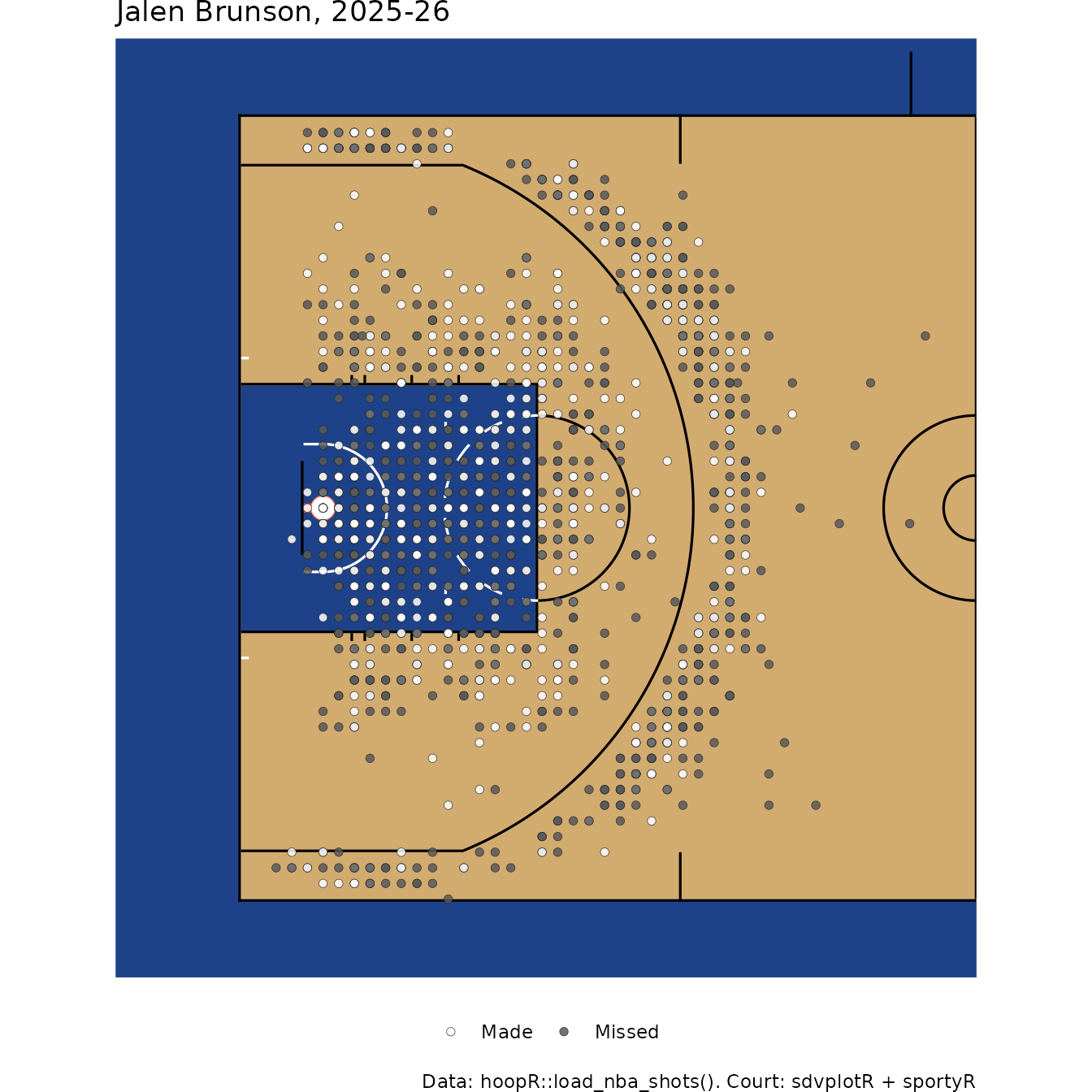

The same half-court shot chart drawn on a court painted in the player's team colors.

Where do shots come from? Hexbin maps

With hundreds of overlapping points a scatter plot saturates. A hexbin map counts attempts in small hexagons instead. Here is the whole league, which needs the hexbin package:

league_shots <- nba_shots |>
  mutate(
    right = coordinate_x > 0,
    x = if_else(right, -coordinate_x, coordinate_x),
    y = if_else(right, -coordinate_y, coordinate_y)
  ) |>
  filter(x <= 0)

geom_basketball("nba", display_range = "defense") +
  geom_hex(aes(x, y), data = league_shots, binwidth = c(1.5, 1.5), alpha = 0.85) +
  scale_fill_viridis_c(trans = "log10", name = "Attempts") +
  labs(title = "Where NBA shots came from, 2025-26",
       subtitle = sprintf("%s field-goal attempts", format(nrow(league_shots), big.mark = ",")),
       caption = "Data: hoopR::load_nba_shots()")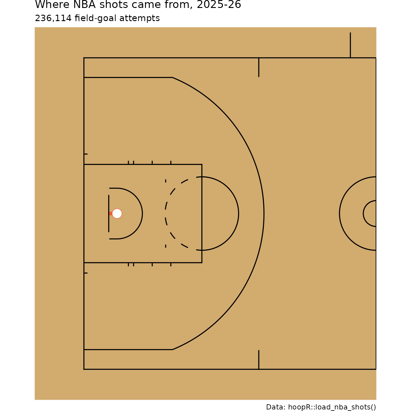

Hexbin map of every NBA field-goal attempt in 2025-26 on a half court, colored by the log count of attempts, showing clusters at the rim and beyond the three-point line.

The two clusters, at the rim and just beyond the three-point line, are the modern shot profile: the mid-range is comparatively empty. Coloring each hexagon by its make rate instead of its count shows efficiency by location (stat_summary_hex() averages z in each bin):

geom_basketball("nba", display_range = "defense") +
  stat_summary_hex(
    aes(x, y, z = as.numeric(scoring_play)), data = league_shots,
    fun = \(z) if (length(z) >= 30) mean(z) else NA_real_,
    binwidth = c(2, 2), alpha = 0.9
  ) +
  scale_fill_distiller(palette = "RdBu", direction = 1, limits = c(0.2, 0.8),
                       oob = scales::squish, name = "FG%", na.value = NA) +
  labs(title = "NBA field-goal percentage by location, 2025-26",
       subtitle = "Hexagons with at least 30 attempts",
       caption = "Data: hoopR::load_nba_shots()")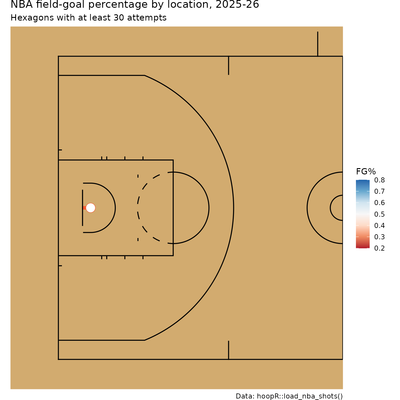

Hexbin map of NBA field-goal percentage by court location in 2025-26, limited to hexagons with at least 30 attempts.

Smooth density maps

A two-dimensional kernel density estimate smooths the same information into contours, which reads well for a single player:

geom_basketball("nba", display_range = "defense") +
  stat_density_2d_filled(aes(x, y), data = player_shots, alpha = 0.7,
                         contour_var = "ndensity", bins = 8) +
  scale_fill_brewer(palette = "Blues", guide = "none") +
  labs(title = paste0(volume$athlete_name_1, ": shot density, 2025-26"),
       caption = "Data: hoopR::load_nba_shots()")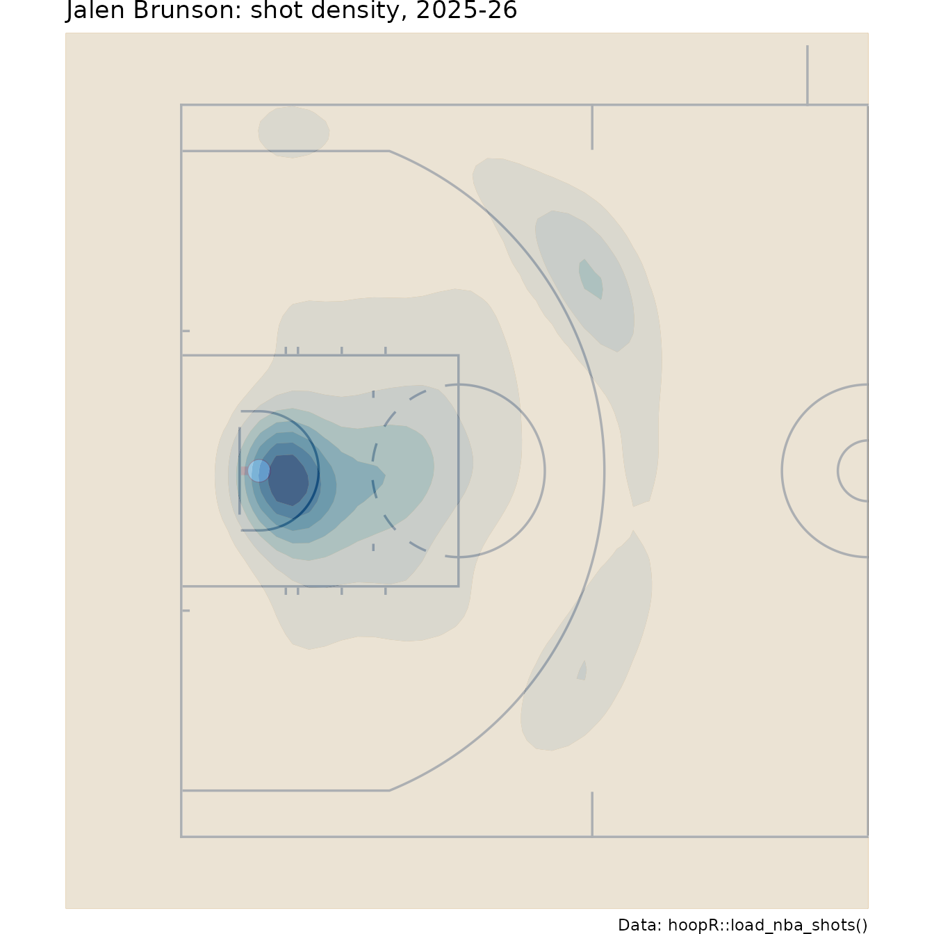

Filled density contours of the selected NBA player's shot locations on a half court.

Shot zones and FG% by zone

Zones turn a chart into a table. A standard five-zone split:

Restricted area: within 4 feet of the basket.
Paint (non-restricted area): the rest of the lane (16 feet wide in the NBA, 12 in college, 19 feet deep from the baseline).
Mid-range: every other two-point attempt.
Corner 3: three-pointers from the straight part of the line along the sideline.
Above-the-break 3: every other three.

Zone boundaries need to know whether an attempt was a three. ESPN’s NBA shot file records score_value = 0 for misses, so it cannot tell a missed three from a missed two. The NBA Stats file can: shot_value is the attempt’s value. We use load_nba_stats_shots() (note it takes the season’s start year) and convert its legacy coordinates with sdv_court_coords(), which divides by ten and moves the origin to center court so the shots fit geom_basketball().

# Approximate zone geometry on sportyR's frame (basket at x = -41.75, feet).
shot_zone <- function(x, y, is_three, paint_half_width = 8, corner_depth = 14) {
  dist <- sqrt((x + 41.75)^2 + y^2)
  case_when(
    is_three & x <= -47 + corner_depth & abs(y) >= 20 ~ "Corner 3",
    is_three ~ "Above-the-break 3",
    dist <= 4 ~ "Restricted area",
    abs(y) <= paint_half_width & x <= -47 + 19 ~ "Paint (non-RA)",
    TRUE ~ "Mid-range"
  )
}
zone_levels <- c("Restricted area", "Paint (non-RA)", "Mid-range", "Corner 3", "Above-the-break 3")

stats_shots <- load_nba_stats_shots(seasons = season - 1) |>
  as.data.frame() |>
  sdvplotR::sdv_court_coords(x_column = "x_legacy", y_column = "y_legacy") |>
  filter(season_type_id == 2) |>                      # regular season
  mutate(
    made = shot_result == "Made",
    zone = factor(shot_zone(court_x, court_y, shot_value == 3), levels = zone_levels)
  )

league_zones <- stats_shots |>
  group_by(zone) |>
  summarise(fga = n(), fg_pct = mean(made), pts_per_shot = mean(made * shot_value)) |>
  mutate(share = fga / sum(fga))

league_zones |>
  mutate(across(c(fg_pct, pts_per_shot, share), \(x) round(x, 3)))
#> # A tibble: 5 × 5
#>   zone                fga fg_pct pts_per_shot share
#>   <fct>             <int>  <dbl>        <dbl> <dbl>
#> 1 Restricted area   62278  0.671        1.34  0.284
#> 2 Paint (non-RA)    43714  0.446        0.891 0.199
#> 3 Mid-range         22197  0.416        0.833 0.101
#> 4 Corner 3          23577  0.387        1.16  0.108
#> 5 Above-the-break 3 67393  0.35         1.05  0.308

Points per shot (FG% times the shot’s value) is the fair comparison across zones: a three only needs to go in two-thirds as often as a two to be worth the same.

Now one player against the league. We take the NBA Stats leader in field-goal attempts (its player_name is a short name):

target <- stats_shots |>
  count(person_id, player_name, sort = TRUE) |>
  slice_head(n = 1)
target
#>   person_id player_name    n
#> 1   1627759       Brown 1543

player_zones <- stats_shots |>
  filter(person_id == target$person_id) |>
  group_by(zone) |>
  summarise(fga = n(), fg_pct = mean(made)) |>
  left_join(select(league_zones, zone, league_fg_pct = fg_pct), by = "zone") |>
  mutate(diff = fg_pct - league_fg_pct)

player_zones |>
  mutate(across(c(fg_pct, league_fg_pct, diff), \(x) round(x, 3)))
#> # A tibble: 5 × 5
#>   zone                fga fg_pct league_fg_pct   diff
#>   <fct>             <int>  <dbl>         <dbl>  <dbl>
#> 1 Restricted area     346  0.688         0.671  0.017
#> 2 Paint (non-RA)      426  0.486         0.446  0.04 
#> 3 Mid-range           367  0.411         0.416 -0.005
#> 4 Corner 3             50  0.38          0.387 -0.007
#> 5 Above-the-break 3   354  0.342         0.35  -0.008

player_zones |>
  tidyr::pivot_longer(c(fg_pct, league_fg_pct), names_to = "who", values_to = "pct") |>
  mutate(who = if_else(who == "fg_pct", target$player_name, "League")) |>
  ggplot(aes(zone, pct, fill = who)) +
  geom_col(position = "dodge", width = 0.7) +
  scale_y_continuous(labels = scales::percent) +
  scale_fill_manual(values = c("#2C3D50", "#A7C6E6"), name = NULL) +
  labs(title = "FG% by shot zone vs league average, 2025-26 regular season",
       x = NULL, y = "FG%", caption = "Data: hoopR::load_nba_stats_shots()") +
  theme_minimal() +
  theme(legend.position = "bottom")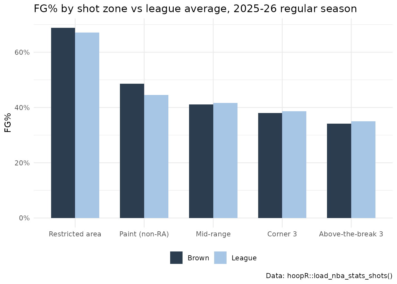

Bar chart comparing the selected player's field-goal percentage with the NBA league average in each of five shot zones.

And the zones drawn on the court, to check the geometry:

geom_basketball("nba", display_range = "defense") +
  geom_point(aes(court_x, court_y, colour = zone),
             data = filter(stats_shots, person_id == target$person_id),
             size = 1.2, alpha = 0.7) +
  scale_colour_brewer(palette = "Set2", name = NULL) +
  labs(title = paste0(target$player_name, ": shots by zone, 2025-26"),
       caption = "Data: hoopR::load_nba_stats_shots(); coordinates via sdvplotR::sdv_court_coords()") +
  theme(legend.position = "bottom")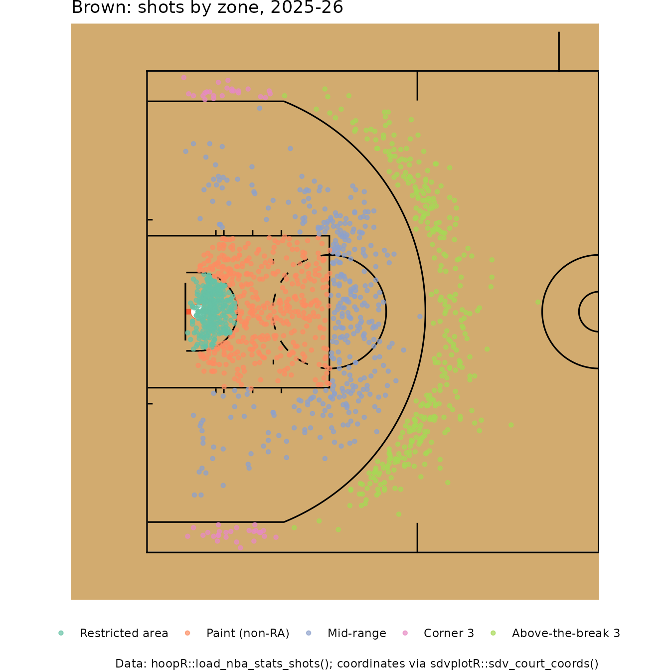

Half-court map of the selected player's shots colored by the five shot zones.

A men’s college basketball shot chart

load_mbb_shots() uses the same ESPN frame as the NBA file, and the college court has the same 94-foot floor and basket position, so the code barely changes. Two differences: the college file has a few placeholder coordinates far off the court, which we drop, and its score_value is the attempt’s value (2 or 3) even for misses, so zones work directly.

mbb_shots <- load_mbb_shots(seasons = season) |>
  filter(!grepl("FreeThrow", type_text),
         abs(coordinate_x) <= 47, abs(coordinate_y) <= 25) |>
  mutate(
    right = coordinate_x > 0,
    x = if_else(right, -coordinate_x, coordinate_x),
    y = if_else(right, -coordinate_y, coordinate_y),
    made = scoring_play,
    # college paint is 12 ft wide; the straight part of the arc is about 10 ft deep
    zone = factor(shot_zone(x, y, score_value == 3, paint_half_width = 6, corner_depth = 10),
                  levels = zone_levels)
  )

mbb_volume <- mbb_shots |>
  count(athlete_id_1, athlete_name_1, team_abbrev, name = "fga", sort = TRUE) |>
  slice_head(n = 1)
mbb_volume
#> # A tibble: 1 × 4
#>   athlete_id_1 athlete_name_1 team_abbrev   fga
#>          <int> <chr>          <chr>       <int>
#> 1      5107508 Kenyon Giles   WICH          610

mbb_player <- filter(mbb_shots, athlete_id_1 == mbb_volume$athlete_id_1)

geom_basketball("ncaa", display_range = "defense") +
  geom_point(aes(x, y, shape = made, colour = made), data = mbb_player,
             size = 1.8, alpha = 0.75) +
  scale_shape_manual(values = c(`TRUE` = 16, `FALSE` = 4), labels = c("Missed", "Made"), name = NULL) +
  scale_colour_manual(values = c(`TRUE` = "#2C3D50", `FALSE` = "grey45"), labels = c("Missed", "Made"), name = NULL) +
  labs(title = paste0(mbb_volume$athlete_name_1, " (", mbb_volume$team_abbrev, "), 2025-26"),
       subtitle = sprintf("%d field-goal attempts, %.1f%% FG", nrow(mbb_player), 100 * mean(mbb_player$made)),
       caption = "Data: hoopR::load_mbb_shots() (ESPN). Court: sportyR") +
  theme(legend.position = "bottom")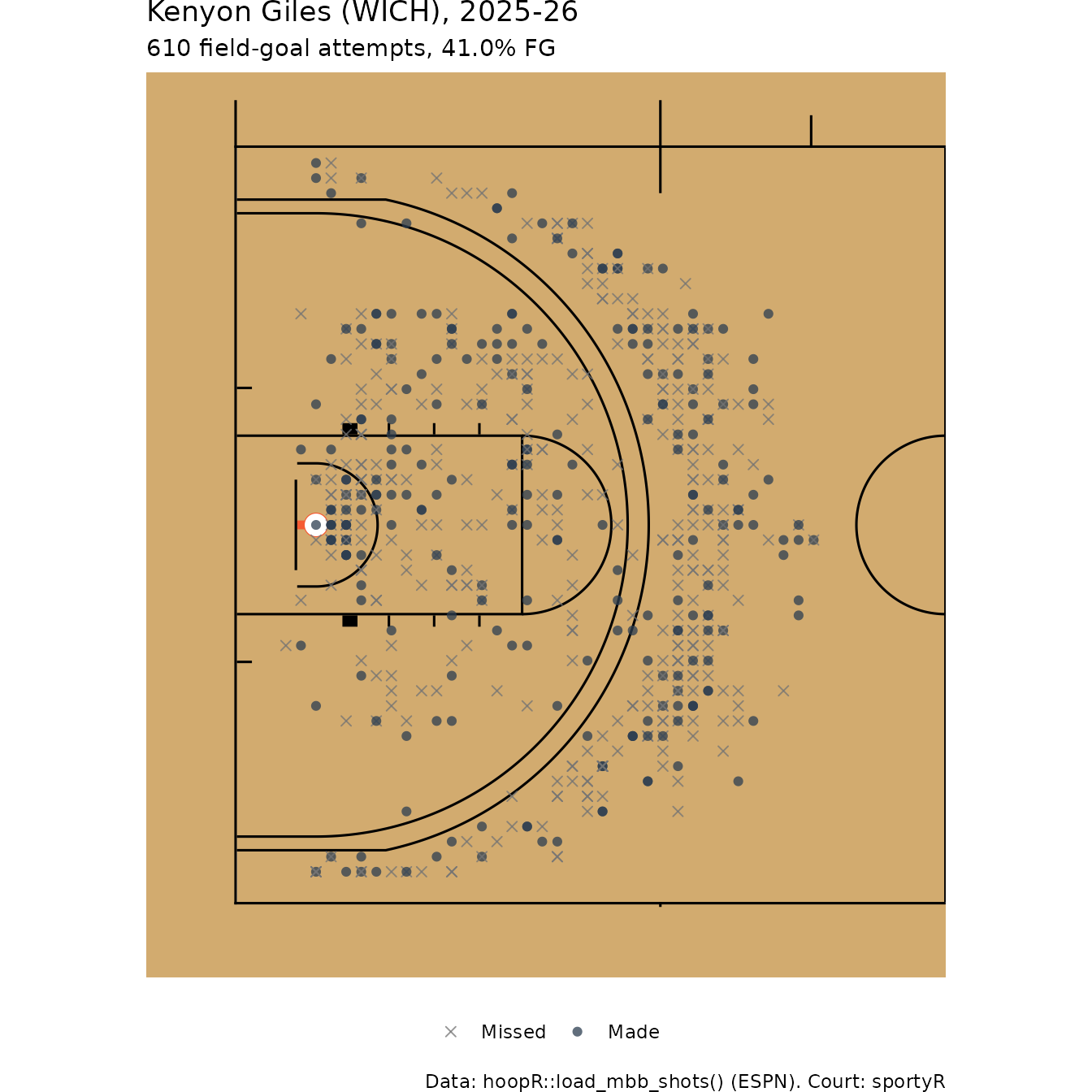

Half-court college basketball shot chart for the 2025-26 Division I leader in field-goal attempts, with makes and misses distinguished.

How does the college shot profile compare with the NBA’s?

mbb_zones <- mbb_shots |>
  group_by(zone) |>
  summarise(fga = n(), fg_pct = mean(made)) |>
  mutate(share = fga / sum(fga))

bind_rows(
  mutate(league_zones, league = "NBA"),
  mutate(mbb_zones, league = "Men's college")
) |>
  select(league, zone, share, fg_pct) |>
  mutate(across(c(share, fg_pct), \(x) round(x, 3))) |>
  tidyr::pivot_wider(names_from = league, values_from = c(share, fg_pct))
#> # A tibble: 5 × 5
#>   zone         share_NBA `share_Men's college` fg_pct_NBA `fg_pct_Men's college`
#>   <fct>            <dbl>                 <dbl>      <dbl>                  <dbl>
#> 1 Restricted …     0.284                 0.253      0.671                  0.649
#> 2 Paint (non-…     0.199                 0.243      0.446                  0.452
#> 3 Mid-range        0.101                 0.109      0.416                  0.365
#> 4 Corner 3         0.108                 0.074      0.387                  0.36 
#> 5 Above-the-b…     0.308                 0.322      0.35                   0.333

Caveats

Coordinates are charted by people. ESPN and NBA Stats locations are recorded in-arena or from video and can be off by a foot or two; heaves and tip-ins near the rim are noisy.
Zone boundaries here are approximate. The geometry above uses round numbers; the official three-point line has a slightly different corner depth, and shots on a line can land in either zone. Use the NBA Stats shot_value (or college score_value) for whether a shot was a three, never distance alone.
Small samples. FG% in a zone with a few dozen attempts is noisy. Filter hexagons and zones by attempt counts, as above.
Frames. Never pass ESPN coordinate_x / coordinate_y to sdv_court_coords(); it is for the NBA Stats legacy frame (and EuroLeague’s, with provider = "euroleague").

Where to go next

The advanced metrics article turns shooting into eFG% and true shooting.
sdvplotR’s own shot chart cookbook has more court styles, plus NBA and men’s college visualization guides.
International shot data: EuroLeague’s euroleague_game_points() and many league *_shots() functions, covered in the international leagues guide.
Reference pages: load_nba_shots(), load_mbb_shots(), load_nba_stats_shots() and load_ncaa_mbb_shots() in the hoopR Data section.

Saiem Gilani