College Basketball RAPM Model: Regularized Adjusted Plus-Minus for NCAA Men's Players

Regularized adjusted plus-minus (RAPM) asks one question of every possession: given the ten players on the floor, how many points did it produce, and how much of that belongs to each player? Solve that jointly over a whole season and each player’s coefficient is his estimated effect on a possession, controlling for every teammate and opponent he shared the floor with. hoopR serves two college RAPM datasets built this way, load_ncaa_mbb_rapm() (league-wide) and load_ncaa_mbb_rapm_within_team() (within-team), and its nba_rapm() function lets you fit the same kind of model yourself. This article explains all three.

The official model card for the college ratings is rapm.md in the ncaa-mbb-hoops-data repository. Numbers below are either computed in this article from the published releases or quoted from the card and labeled “as reported in the model card”.

Plus-minus, APM and RAPM

Plus-minus is a team’s point differential while a player is on the floor. It is easy to compute and badly confounded: a bench player who always plays beside an All-American looks great.
Adjusted plus-minus (APM) fixes the confounding with a regression. Each row is a possession (or a stint of possessions), each player gets an indicator column, and the outcome is points scored. The coefficients separate each player’s contribution from his teammates’ and opponents’.
Regularized APM (RAPM) adds a ridge penalty. Plain APM is wildly unstable because players who share the floor are nearly collinear and many have few possessions. The ridge penalty shrinks every coefficient toward zero, more strongly the less data a player has, trading a little bias for a large drop in variance.

Two estimands, never merged

	League-wide RAPM	Within-team RAPM
Loader	`load_ncaa_mbb_rapm()`	`load_ncaa_mbb_rapm_within_team()`
Fit	One ridge regression over all Division I possessions of a season	One fit per team, over that team’s own possessions
Scale	Points per 100 possessions, comparable across teams	Apportions one team’s performance across its players; not comparable across teams
Columns	`orapm`, `drapm`, `rapm_net`, `off_poss`, `def_poss`, `estimand`	`rapm_off`, `rapm_def`, `rapm_net`, `team_off_poss`, `num_players`
Coverage	Seasons 2011 to 2026	See the reference page

Every league-wide row carries estimand = "league" so the two cannot be silently mixed.

How is the league-wide model fit?

As described in the model card:

Design. Each row is a possession. Each player has a column that is +1 when he is on offense and -1 when he is on defense, plus an intercept (the league’s points per 100 possessions) and a home-court term. Offensive and defensive components are estimated jointly; rapm_net = orapm + drapm.
Penalty. Ridge regression with lambda = 1000, fixed by a validation program and asserted at run time, so a fit that silently ran unregularized cannot be published.
Inputs. Possessions compiled by the SportsDataverse NCAA play-by-play engine from stats.ncaa.org, team rosters, and a name-change table that keeps a player in one column across transfers and spelling variants. Season 2010 fails the usable-possession gate and is excluded.
Feature engineering lives in the possessions. Substitution windows, possession trimming, and free-throw and end-of-period edge cases are handled when possessions are built, not in the regression.

What do the inputs look like?

The possession and stint frames the model is built from are published too. Each possession row lists both teams’ five players, points, and flags such as garbage time:

library(hoopR)
library(dplyr)
library(ggplot2)

season <- 2026
poss <- load_ncaa_mbb_possessions(seasons = season)
stints <- load_ncaa_mbb_matchup_stints(seasons = season)

tibble(
  possessions = nrow(poss),
  games = n_distinct(poss$contest_id),
  points_per_100 = round(100 * mean(poss$pts, na.rm = TRUE), 1),
  garbage_time_share = round(mean(poss$is_garbage_time == 1, na.rm = TRUE), 3),
  n_stints = nrow(stints),
  median_stint_possessions = median(stints$n_possessions, na.rm = TRUE)
)
#> # A tibble: 1 × 6
#>   possessions games points_per_100 garbage_time_share n_stints
#>         <int> <int>          <dbl>              <dbl>    <int>
#> 1      878168  6291           108.              0.034   210508
#> # ℹ 1 more variable: median_stint_possessions <dbl>

A stint is a stretch during which the same ten players are on the floor. Stints are short, which is exactly why RAPM needs a full season and a penalty.

What does the league-wide rating look like?

rapm <- load_ncaa_mbb_rapm(seasons = season)

rapm |>
  summarise(
    players = n(),
    median_off_poss = median(off_poss),
    mean_rapm_net = round(mean(rapm_net), 3),
    sd_rapm_net = round(sd(rapm_net), 2)
  )
#> # A tibble: 1 × 4
#>   players median_off_poss mean_rapm_net sd_rapm_net
#>     <int>           <dbl>         <dbl>       <dbl>
#> 1    4974            758.             0        2.78

Shrinkage is visible directly: players with few possessions sit near zero because the data cannot separate them from their lineups, and the spread widens as possessions accumulate.

ggplot(rapm, aes(off_poss, rapm_net)) +
  geom_hline(yintercept = 0, colour = "grey70") +
  geom_point(alpha = 0.2, size = 0.8, colour = "#2C3D50") +
  labs(
    title = "Ridge shrinkage: low-possession players are pulled toward zero",
    subtitle = "League-wide NCAA men's RAPM, 2025-26",
    x = "Offensive possessions", y = "RAPM (points per 100 possessions)",
    caption = "Data: hoopR::load_ncaa_mbb_rapm()"
  ) +
  theme_minimal()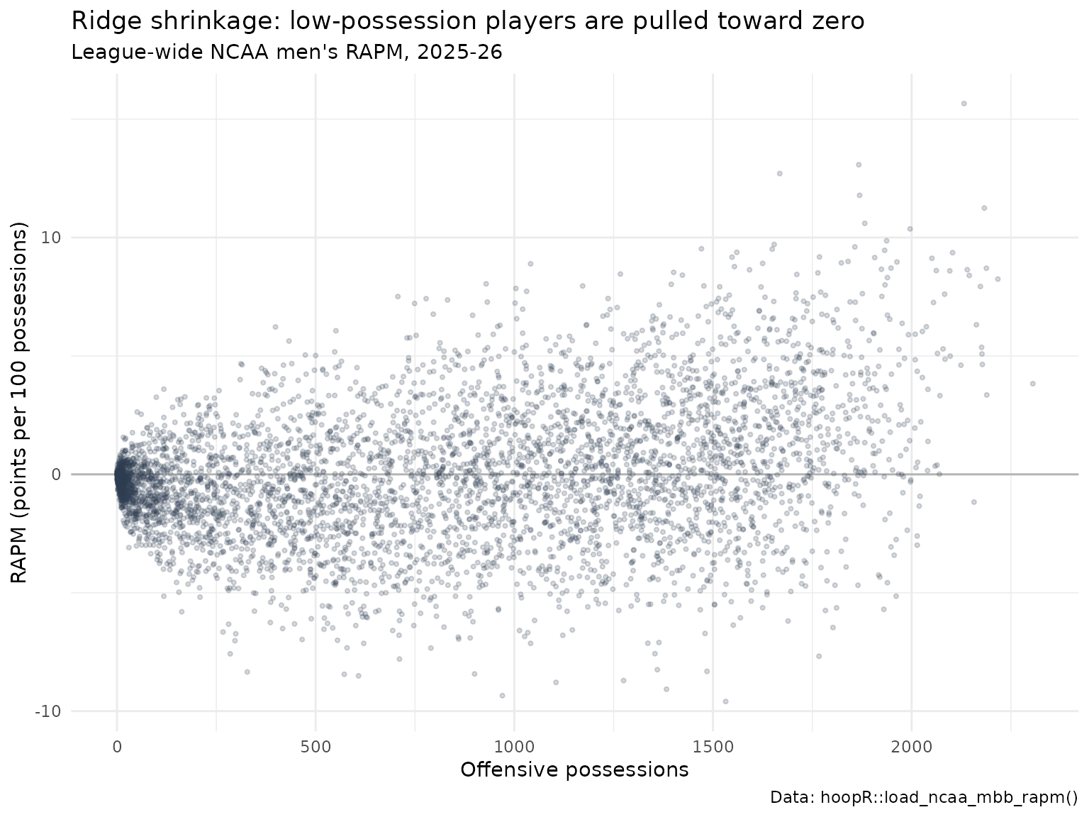

Scatter plot of league-wide college RAPM against offensive possessions for 2025-26, showing estimates near zero for low-possession players and a wider spread for high-possession players.

The leaders, with a possession floor so the list is not dominated by noise:

rapm |>
  filter(off_poss >= 800) |>
  arrange(desc(rapm_net)) |>
  select(player, team, off_poss, orapm, drapm, rapm_net) |>
  mutate(across(orapm:rapm_net, \(x) round(x, 2))) |>
  head(15)
#> # A tibble: 15 × 6
#>    player           team           off_poss orapm drapm rapm_net
#>    <chr>            <chr>             <int> <dbl> <dbl>    <dbl>
#>  1 YAXEL.LENDEBORG  Michigan           2132  8.7   6.96    15.7 
#>  2 FLORY.BIDUNGA    Kansas             1867  5.1   7.97    13.1 
#>  3 HENRI.VEESAAR    North Carolina     1668  6.24  6.47    12.7 
#>  4 MJ.COLLINS       Utah St.           1869  6.84  4.94    11.8 
#>  5 JAKOBI.GILLESPIE Tennessee          2183  9.17  2.08    11.2 
#>  6 FLETCHER.LOYER   Purdue             1882  5.96  4.64    10.6 
#>  7 KEATON.WAGLER    Illinois           1996  7.65  2.71    10.4 
#>  8 JEREMY.FEARS     Michigan St.       1937  4.21  5.65     9.86
#>  9 ROBBIE.AVILA     Saint Louis        1654  6.02  3.68     9.71
#> 10 JOSHUA.JEFFERSON Iowa St.           1857  5.8   3.81     9.6 
#> 11 DAME.SARR        Duke               1471  3.22  6.31     9.53
#> 12 IZAIYAH.NELSON   South Fla.         1649  4.23  5.28     9.51
#> 13 MILAN.MOMCILOVIC Iowa St.           1932  3.79  5.67     9.46
#> 14 TREY.MCKENNEY    Michigan           1560  4.25  5.12     9.38
#> 15 CAMERON.BOOZER   Duke               2103  6.46  2.9      9.36

Standard errors

The model card documents ridge posterior standard errors in orapm_se, drapm_se and rapm_net_se, so rapm_net ± 2 * rapm_net_se gives a deliberately cautious band. The asset load_ncaa_mbb_rapm(2026) returned when this article was built does not include these columns yet, so check names() on what you load. As reported in the model card, the posterior SE is about 4 points per 100 for high-possession players and about 5 for the lowest-possession players, and a split-half test shows it is conservative by roughly 2.5 times relative to how much an estimate moves between two halves of a season. At the top of the leaderboard the bands overlap almost entirely: treat it as a tier, not a ranking.

Within-team versus league-wide

The within-team fit answers a different question, so the two should agree only partly:

within <- load_ncaa_mbb_rapm_within_team(seasons = season)

both <- rapm |>
  select(player_id, player, team, off_poss, rapm_net) |>
  inner_join(within |> select(player_id, rapm_net_within = rapm_net), by = "player_id") |>
  filter(off_poss >= 500)

c(players = nrow(both), r = round(cor(both$rapm_net, both$rapm_net_within), 3))
#> players       r 
#> 3026.00    0.83

How well does it validate?

RAPM has no ground truth to score against, so validation checks that the fit is on the right scale and that it aggregates to sensible team strengths.

As reported in the model card, every season 2011-2026 passes publish-blocking gates: at least 65% of possessions usable (observed minimum 0.7414); an intercept between 95 and 112 points per 100 (observed 99.24 to 107.97); a home-court term between 1 and 4 points; and a Spearman correlation between a possession-weighted team aggregate and Bart Torvik’s adjusted efficiency margin of 0.943 to 0.978 by season. The intercept and home-court bands catch scale bugs that a rank correlation cannot see.

We can run a similar team-level check here against the SportsDataverse’s own opponent-adjusted team ratings (load_mbb_ratings(), explained in the team ratings article). Each team’s possession-weighted mean of player RAPM is a rough proxy for team strength; the possession file maps NCAA team names to ESPN team ids:

ratings <- load_mbb_ratings(seasons = season)

if (nrow(ratings) > 0) {
  team_map <- poss |>
    distinct(team = poss_team, team_id = as.character(poss_team_espn_team_id)) |>
    filter(!is.na(team_id))

  proxy <- rapm |>
    group_by(team) |>
    summarise(team_rapm = weighted.mean(rapm_net, off_poss + def_poss), .groups = "drop") |>
    inner_join(team_map, by = "team") |>
    inner_join(ratings |> transmute(team_id = as.character(team_id), adj_em), by = "team_id")

  c(teams = nrow(proxy),
    spearman = round(cor(proxy$team_rapm, proxy$adj_em, method = "spearman"), 3))
}
#>    teams spearman 
#>   365.00     0.98

This proxy is not the model card’s gate statistic, and the reference ratings are a different model, so treat it as a sanity check rather than a validation result. It validates team-level aggregation, not the ordering of individual players.

Fit your own RAPM in R with nba_rapm()

hoopR also ships an in-package RAPM fitter, nba_rapm(), that works on any possession frame with off_player_1 to off_player_5, def_player_1 to def_player_5 and points. Its design, read directly from the code:

Design matrix: for P players, 2P sparse indicator columns. Column j is 1 when player j is on offense; column P + j is 1 when he is on defense. Possessions with any missing lineup slot are dropped.
Model: ridge regression (glmnet, alpha = 0) with no intercept. The penalty is chosen by 10-fold cross-validation at lambda.min, with deterministic folds (every tenth possession), so results are reproducible without a seed.
Output: o_rapm is the offensive coefficient times 100, d_rapm is minus the defensive coefficient times 100 (so good defense is positive), rapm = o_rapm + d_rapm, plus possession counts.

The SportsDataverse’s NBA possession frame, load_nba_stats_possessions(), has exactly those columns, so a full NBA regular season fits offline in seconds. (Note this loader takes the season’s start year; game_ids starting with 002 are regular-season games.) nba_rapm() needs the glmnet and Matrix packages.

nba_poss <- load_nba_stats_possessions(seasons = 2025) |>
  filter(substr(game_id, 1, 3) == "002")

c(possessions = nrow(nba_poss), games = n_distinct(nba_poss$game_id))
#> possessions       games 
#>      245646        1230

fit_time <- system.time(my_rapm <- nba_rapm(nba_poss))
round(fit_time[["elapsed"]], 1)
#> [1] 12

my_rapm |>
  summarise(players = n(), mean_o_rapm = mean(o_rapm), mean_d_rapm = mean(d_rapm),
            mean_rapm = mean(rapm)) |>
  mutate(across(-players, \(x) round(x, 2)))
#> # A tibble: 1 × 4
#>   players mean_o_rapm mean_d_rapm mean_rapm
#>     <int>       <dbl>       <dbl>     <dbl>
#> 1     582        10.1       -11.7     -1.58

Two properties of this design show up immediately:

No intercept, so the league average lives in the players. About one point per possession has to come from somewhere, and with no intercept it is split across the ten player coefficients on every possession. That is why mean o_rapm is well above zero and mean d_rapm well below. The sum rapm is roughly centered, but compare o_rapm and d_rapm only after centering them.
Cross-validated lambda is light. lambda.min is chosen for predicting possession outcomes, and it regularizes far less than the college model’s lambda = 1000. Players with a few dozen possessions get extreme values. Use a possession floor.

Compare with the published suite’s RAPM for the same season:

published <- load_nba_player_impact(seasons = 2026) |>
  filter(season_type == "Regular Season") |>
  select(player_id, player_name, rapm_published = rapm)

compare <- my_rapm |>
  inner_join(published, by = "player_id") |>
  mutate(o_centered = o_rapm - weighted.mean(o_rapm, off_poss),
         d_centered = d_rapm - weighted.mean(d_rapm, def_poss))

compare |>
  mutate(floor = if_else(off_poss >= 1000, "1,000+ possessions", "under 1,000")) |>
  group_by(floor) |>
  summarise(players = n(), r_with_published = round(cor(rapm, rapm_published), 3))
#> # A tibble: 2 × 3
#>   floor              players r_with_published
#>   <chr>                <int>            <dbl>
#> 1 1,000+ possessions     384            0.955
#> 2 under 1,000            198            0.452

compare |>
  filter(off_poss >= 1000) |>
  ggplot(aes(rapm_published, rapm)) +
  geom_abline(colour = "grey70", linetype = "dashed") +
  geom_point(alpha = 0.6, colour = "#2C3D50") +
  labs(
    title = "nba_rapm() vs the published RAPM, 2025-26 regular season",
    subtitle = "Players with 1,000+ offensive possessions",
    x = "Published RAPM (load_nba_player_impact)", y = "nba_rapm() fit",
    caption = "Data: hoopR::load_nba_stats_possessions(), hoopR::load_nba_player_impact()"
  ) +
  theme_minimal()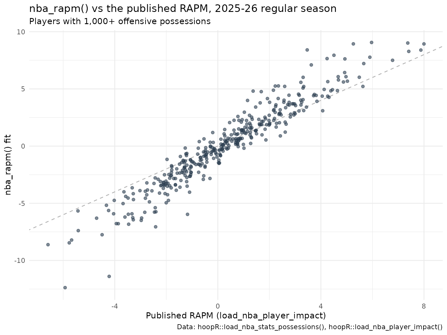

Scatter plot comparing RAPM fitted with nba_rapm() against the published NBA player impact RAPM for players with at least 1,000 offensive possessions in 2025-26.

For regulars the two agree closely in ordering; the scale differs because the published suite regularizes more heavily and centers its components. To control the penalty yourself, build the design and call glmnet::glmnet() with your own lambda, or add an intercept.

For a single game you can build the possession frame from live NBA Stats play-by-play with nba_possession_lineups(). It calls stats.nba.com, so it is not run here, and one game (about 200 possessions) is far too few for a meaningful RAPM:

one_game <- nba_possession_lineups(game_id = "0022200001")
nba_rapm(one_game)   # pipeline illustration only

The same approach works for college: load_ncaa_mbb_possessions() lists the ten players by stats.ncaa.org player id (home_1_player_id … away_5_player_id) with pts and poss_team, which you can reshape into offense/defense columns.

Limitations

Retrodictive, not predictive. RAPM describes what happened on the floor. As reported in the model card, single-season college RAPM predicts next season’s RAPM for returning players only modestly (Spearman about 0.31 for the single-season baseline).
Collinearity. Players who always share the floor are separated only by the prior.
Low-possession shrinkage. Low-minute players are pulled toward zero; a near-zero RAPM can mean “average” or “unknown”.
Not luck-adjusted. Opponent three-point shooting luck is not removed from the target yet.
Within-team is not cross-team. Do not compare load_ncaa_mbb_rapm_within_team() values between teams.
Names and ids. League-wide player is LAST.FIRST; join on player_id (stats.ncaa.org) or person_id (stable across seasons and teams).

Where to go next

NBA player impact model: RAPM with SPM priors, BPM, DARKO-style projections and WAR.
College basketball player value model: the box-score counterpart to RAPM.
College basketball team ratings model and win probability model.
Basketball advanced metrics for possessions and ratings.
Reference: the NCAA engine loaders and nba_rapm().

Saiem Gilani