Basketball Advanced Metrics in R: Possessions, Pace, Ratings and the Four Factors

Points per game tells you how much a team scored. Points per possession tells you how well it scored. This article walks through the standard efficiency metrics of basketball analytics, shows the formula for each, computes it with hoopR’s helpers on a full NBA season, and checks the helper against a hand calculation. Everything here runs offline on the SportsDataverse release files, so it is fast and reproducible.

If you are new to hoopR, start with Getting Started with hoopR. The helpers used here live in the Basketball Analytics Utilities section of the reference.

What you need

library(hoopR)
library(dplyr)
library(ggplot2)

season <- 2026 # the 2025-26 season

We use three release loaders: load_nba_team_box() (one row per team per game), load_nba_player_box() (one row per player per game) and load_nba_pbp() (to count overtime periods). Team box scores carry ESPN’s column names, so we rename them once to the short names the helpers expect.

team_box <- load_nba_team_box(seasons = season) |>
  filter(season_type == 2) |>                       # regular season
  add_count(team_id, name = "team_games") |>
  filter(team_games >= 41) |>                       # drop All-Star exhibition teams
  transmute(
    game_id, team_id, team = team_abbreviation, opp_id = opponent_team_id,
    pts = team_score, fgm = field_goals_made, fga = field_goals_attempted,
    fg3m = three_point_field_goals_made, fg3a = three_point_field_goals_attempted,
    ftm = free_throws_made, fta = free_throws_attempted,
    oreb = offensive_rebounds, dreb = defensive_rebounds,
    ast = assists, tov = total_turnovers
  )

# minutes played: 48 per regulation game plus 5 per overtime period
game_minutes <- load_nba_pbp(seasons = season) |>
  group_by(game_id) |>
  summarise(periods = max(period_number), .groups = "drop") |>
  mutate(game_min = 48 + 5 * pmax(periods - 4, 0))

# attach each team's opponent totals to its own row
games <- team_box |>
  inner_join(
    team_box |> select(game_id, opp_id = team_id, opp_pts = pts, opp_fgm = fgm,
                       opp_fga = fga, opp_fg3m = fg3m, opp_ftm = ftm, opp_fta = fta,
                       opp_oreb = oreb, opp_dreb = dreb, opp_tov = tov),
    by = c("game_id", "opp_id")
  ) |>
  inner_join(game_minutes, by = "game_id")

# a few box scores have missing team totals; drop those team-games
n_before <- nrow(games)
games <- filter(games, if_all(everything(), \(x) !is.na(x)))
c(team_games = nrow(games), dropped_incomplete = n_before - nrow(games))
#>         team_games dropped_incomplete 
#>               2458                  2

How many possessions did a team have?

A possession is one team’s turn with the ball. It ends with a made field goal (or last free throw), a defensive rebound, a turnover, or the end of a period. An offensive rebound extends a possession rather than starting a new one. Box scores do not record possessions, so we estimate them:

possessions = FGA + 0.44 * FTA - OREB + TOV

nba_possessions() computes exactly that. The 0.44 is the average share of a possession a free-throw attempt ends: two-shot fouls use two attempts for one possession, three-shot fouls three, and and-ones and technicals add attempts that end nothing.

Both teams in a game have (almost) the same number of possessions, so a common refinement averages the two estimates. We use that game-level average for every rating below.

games <- games |>
  mutate(
    poss_own = nba_possessions(fga, fta, oreb, tov),
    poss_opp = nba_possessions(opp_fga, opp_fta, opp_oreb, opp_tov),
    poss = (poss_own + poss_opp) / 2
  )

# hand check on the first row
g <- games[1, ]
hand <- g$fga + 0.44 * g$fta - g$oreb + g$tov
c(helper = g$poss_own, hand = hand, equal = isTRUE(all.equal(g$poss_own, hand)))
#> helper   hand  equal 
#>  109.2  109.2    1.0

summary(games$poss)
#>    Min. 1st Qu.  Median    Mean 3rd Qu.    Max. 
#>   85.84   98.60  102.24  102.54  105.84  129.88

The two teams’ single-side estimates differ by a median of 2 possessions per game, which is why the average is preferred.

What is pace?

Pace is possessions per 48 minutes. nba_pace() takes the possession count and the team’s total player-minutes (240 for a regulation game, five players times 48 minutes) and returns

pace = 48 * possessions / (minutes / 5)

so overtime games are not mistaken for fast ones.

games <- games |>
  mutate(team_min = 5 * game_min, pace = nba_pace(poss, team_min))

c(helper = games$pace[1], hand = 48 * games$poss[1] / (games$team_min[1] / 5))
#> helper   hand 
#> 107.44 107.44

Offensive, defensive and net rating

Offensive rating (ORtg): points scored per 100 possessions, 100 * PTS / poss, from nba_offensive_rating().
Defensive rating (DRtg): points allowed per 100 possessions, 100 * opponent PTS / poss, from nba_defensive_rating(). Lower is better.
Net rating: ORtg - DRtg, from nba_net_rating(). A net rating of +5 means outscoring opponents by five points every 100 possessions.

Ratings for a season are computed from season totals (sum the points, sum the possessions, then divide), not by averaging game ratings, so long games count for more.

team_season <- games |>
  group_by(team) |>
  summarise(
    gp = n(), pts = sum(pts), opp_pts = sum(opp_pts),
    poss = sum(poss), team_min = sum(team_min),
    .groups = "drop"
  ) |>
  mutate(
    pace = nba_pace(poss, team_min),
    ortg = nba_offensive_rating(pts, poss),
    drtg = nba_defensive_rating(opp_pts, poss),
    net  = nba_net_rating(ortg, drtg)
  ) |>
  arrange(desc(net))

team_season |>
  select(team, gp, pace, ortg, drtg, net) |>
  mutate(across(pace:net, \(x) round(x, 1))) |>
  head(10)
#> # A tibble: 10 × 6
#>    team     gp  pace  ortg  drtg   net
#>    <chr> <int> <dbl> <dbl> <dbl> <dbl>
#>  1 OKC      82 102.   116   105.  10.9
#>  2 DET      82 102.   114.  106.   7.9
#>  3 SA       83 102.   117.  109.   7.9
#>  4 BOS      82  97.7  117.  109.   7.9
#>  5 NY       83  99.4  117.  110.   6.4
#>  6 HOU      82  99    115.  110.   5.2
#>  7 DEN      82 101.   120.  114.   5  
#>  8 CHA      82  99.9  116.  111.   4.8
#>  9 CLE      82 103.   116.  112.   4  
#> 10 MIN      82 103.   114.  110.   3.2

Across the league, teams scored 112.7 points per 100 possessions at a pace of 102 possessions per 48 minutes. Net rating tracks winning closely, which is why it is the headline team metric:

team_season |>
  mutate(margin_pg = (pts - opp_pts) / gp) |>
  ggplot(aes(margin_pg, net, label = team)) +
  geom_abline(slope = 100 / lg_pace, intercept = 0, colour = "grey70", linetype = "dashed") +
  geom_point(colour = "#2C3D50", size = 2.5) +
  geom_text(nudge_y = 0.6, size = 3) +
  labs(
    title = "Net rating is point differential, rescaled to 100 possessions",
    subtitle = "Dashed line: 100 / league pace",
    x = "Point differential per game", y = "Net rating (points per 100 possessions)",
    caption = "Data: hoopR::load_nba_team_box()"
  ) +
  theme_minimal()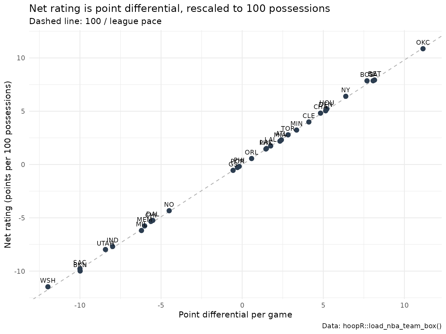

Scatter plot of NBA team net rating against point differential per game for the 2025-26 regular season, showing a near-linear relationship.

The four factors

Dean Oliver identified four things a team must do well to win, on both offense and defense:

Factor	Formula	Helper
Shooting: effective FG%	`(FGM + 0.5 * 3PM) / FGA`	`nba_effective_fg_pct()`
Turnovers: turnover %	`100 * TOV / (FGA + 0.44 * FTA + TOV)`	`nba_turnover_pct()`
Rebounding: offensive rebound %	`100 * OREB / (OREB + opponent DREB)`	`nba_oreb_pct()`
Free throws: free-throw rate	`FTM / FGA`	inside `nba_four_factors()`

Effective field-goal percentage (eFG%) credits a made three with 1.5 field goals, because it is worth 1.5 times a two. Turnover percentage (TOV%) is turnovers per 100 plays. Offensive rebound percentage (OREB%) is the share of a team’s own misses it rebounded. The free-throw rate in the four factors is free throws made per field-goal attempt; the standalone nba_ft_rate() returns the more common attempts-based version, FTA / FGA. Mind which one you report.

nba_four_factors() returns all four as a tibble. The defensive four factors are simply the opponent’s offensive four factors.

ff <- games |>
  group_by(team) |>
  summarise(across(c(fgm, fg3m, fga, fta, ftm, oreb, tov, dreb,
                     opp_fgm, opp_fg3m, opp_fga, opp_fta, opp_ftm, opp_oreb, opp_tov, opp_dreb),
                   sum), .groups = "drop")

off_ff <- with(ff, nba_four_factors(fgm, fg3m, fga, fta, ftm, oreb, tov, opp_dreb))
def_ff <- with(ff, nba_four_factors(opp_fgm, opp_fg3m, opp_fga, opp_fta, opp_ftm, opp_oreb, opp_tov, dreb))
names(def_ff) <- paste0("opp_", names(def_ff))

four_factors <- bind_cols(team = ff$team, off_ff, def_ff) |>
  left_join(select(team_season, team, net), by = "team")

four_factors |>
  arrange(desc(net)) |>
  mutate(across(where(is.numeric), \(x) round(x, 3))) |>
  head(8)
#> # A tibble: 8 × 10
#>   team  efg_pct tov_pct oreb_pct ft_rate opp_efg_pct opp_tov_pct opp_oreb_pct
#>   <chr>   <dbl>   <dbl>    <dbl>   <dbl>       <dbl>       <dbl>        <dbl>
#> 1 OKC     0.561    11.2     22.3   0.213       0.519        14.6         25.6
#> 2 DET     0.546    13.0     30.9   0.223       0.517        14.8         25.8
#> 3 SA      0.558    11.7     26.3   0.215       0.522        11.4         23.0
#> 4 BOS     0.553    11.1     29.2   0.167       0.523        11.4         24.3
#> 5 NY      0.557    12.1     29.6   0.187       0.54         13.0         23.4
#> 6 HOU     0.542    13.3     34.8   0.199       0.53         12.1         25.5
#> 7 DEN     0.577    11.5     23.6   0.237       0.543        10.4         24.7
#> 8 CHA     0.552    13.5     30.5   0.2         0.54         11.6         23.4
#> # ℹ 2 more variables: opp_ft_rate <dbl>, net <dbl>

A hand check of the first team’s offensive eFG% and OREB%:

t1 <- ff[1, ]
c(
  efg_helper = off_ff$efg_pct[1],
  efg_hand = (t1$fgm + 0.5 * t1$fg3m) / t1$fga,
  oreb_helper = off_ff$oreb_pct[1],
  oreb_hand = 100 * t1$oreb / (t1$oreb + t1$opp_dreb)
)
#>  efg_helper    efg_hand oreb_helper   oreb_hand 
#>   0.5537064   0.5537064  24.3506494  24.3506494

How much does each factor matter? Here is the correlation of each offensive and defensive factor with net rating across the 30 teams:

four_factors |>
  summarise(across(c(efg_pct, tov_pct, oreb_pct, ft_rate,
                     opp_efg_pct, opp_tov_pct, opp_oreb_pct, opp_ft_rate),
                   \(x) cor(x, net))) |>
  tidyr::pivot_longer(everything(), names_to = "factor", values_to = "cor_with_net") |>
  arrange(desc(abs(cor_with_net))) |>
  mutate(cor_with_net = round(cor_with_net, 2))
#> # A tibble: 8 × 2
#>   factor       cor_with_net
#>   <chr>               <dbl>
#> 1 opp_efg_pct         -0.9 
#> 2 efg_pct              0.62
#> 3 opp_oreb_pct        -0.56
#> 4 tov_pct             -0.53
#> 5 oreb_pct             0.43
#> 6 opp_ft_rate         -0.35
#> 7 opp_tov_pct          0.26
#> 8 ft_rate              0.15

This season the factor most strongly correlated with net rating is opp_efg_pct (r = -0.9); Oliver’s own weighting ranked shooting first, then turnovers, rebounding and free throws. A linear model of net rating on all eight factors explains 99% of the variance across teams this season (an in-sample fit on 30 teams, so treat it as descriptive).

Player shooting efficiency: eFG% and true shooting

True shooting percentage (TS%) extends eFG% to free throws: points per shooting possession,

TS% = PTS / (2 * (FGA + 0.44 * FTA))

computed by nba_true_shooting_pct(). It is the best single number for scoring efficiency because it counts every way of scoring.

player_box <- load_nba_player_box(seasons = season) |>
  filter(season_type == 2, !did_not_play, minutes > 0) |>
  semi_join(team_box, by = c("game_id", "team_id"))

players <- player_box |>
  group_by(athlete_id, athlete_display_name, team_abbreviation) |>
  summarise(
    gp = n(), min = sum(minutes), pts = sum(points),
    fgm = sum(field_goals_made), fga = sum(field_goals_attempted),
    fg3m = sum(three_point_field_goals_made),
    ftm = sum(free_throws_made), fta = sum(free_throws_attempted),
    tov = sum(turnovers), ast = sum(assists),
    .groups = "drop"
  ) |>
  mutate(
    ts_pct  = nba_true_shooting_pct(pts, fga, fta),
    efg_pct = nba_effective_fg_pct(fgm, fg3m, fga),
    ft_rate = nba_ft_rate(fta, fga)
  )

players |>
  filter(fga >= 800) |>
  arrange(desc(ts_pct)) |>
  select(athlete_display_name, team_abbreviation, pts, fga, fta, ts_pct, efg_pct, ft_rate) |>
  mutate(across(ts_pct:ft_rate, \(x) round(x, 3))) |>
  head(10)
#> # A tibble: 10 × 8
#>    athlete_display_name    team_abbreviation   pts   fga   fta ts_pct efg_pct
#>    <chr>                   <chr>             <int> <int> <int>  <dbl>   <dbl>
#>  1 Jalen Duren             DET                1365   803   430  0.688   0.65 
#>  2 Nikola Jokic            DEN                1799  1132   480  0.67    0.618
#>  3 Shai Gilgeous-Alexander OKC                2117  1321   614  0.665   0.597
#>  4 Zion Williamson         NO                 1302   807   465  0.644   0.6  
#>  5 Kevin Durant            HOU                2026  1376   467  0.641   0.588
#>  6 Kon Knueppel            CHA                1498  1084   226  0.633   0.601
#>  7 Kawhi Leonard           LAC                1813  1258   416  0.629   0.573
#>  8 Victor Wembanyama       SA                 1618  1097   454  0.624   0.567
#>  9 OG Anunoby              NY                 1146   821   226  0.623   0.585
#> 10 Jamal Murray            DEN                1905  1360   390  0.622   0.573
#> # ℹ 1 more variable: ft_rate <dbl>

(A player traded mid-season appears once per team here.)

Usage rate: who finishes the plays?

Usage rate estimates the share of team plays a player “used” (ended with a shot, free throws or a turnover) while on the floor:

USG% = 100 * (FGA + 0.44 * FTA + TOV) * (team minutes / 5) / (minutes * (team FGA + 0.44 * team FTA + team TOV))

nba_usage_rate() needs the team’s totals for the games the player played, so we join team totals to each player game and sum.

team_game_totals <- player_box |>
  group_by(game_id, team_id) |>
  summarise(team_fga = sum(field_goals_attempted), team_fta = sum(free_throws_attempted),
            team_tov = sum(turnovers), .groups = "drop") |>
  inner_join(games |> select(game_id, team_id, team_min), by = c("game_id", "team_id"))

usage <- player_box |>
  inner_join(team_game_totals, by = c("game_id", "team_id")) |>
  group_by(athlete_id, athlete_display_name, team_abbreviation) |>
  summarise(
    min = sum(minutes), fga = sum(field_goals_attempted), fta = sum(free_throws_attempted),
    tov = sum(turnovers), team_fga = sum(team_fga), team_fta = sum(team_fta),
    team_tov = sum(team_tov), team_min = sum(team_min), pts = sum(points),
    .groups = "drop"
  ) |>
  mutate(
    usg = nba_usage_rate(fga, fta, tov, min, team_fga, team_fta, team_tov, team_min),
    ts_pct = nba_true_shooting_pct(pts, fga, fta)
  ) |>
  filter(min >= 1500)

usage |>
  arrange(desc(usg)) |>
  select(athlete_display_name, team_abbreviation, min, usg, ts_pct) |>
  mutate(usg = round(usg, 1), ts_pct = round(ts_pct, 3)) |>
  head(10)
#> # A tibble: 10 × 5
#>    athlete_display_name    team_abbreviation   min   usg ts_pct
#>    <chr>                   <chr>             <dbl> <dbl>  <dbl>
#>  1 Luka Doncic             LAL                2293  38.3  0.616
#>  2 Jaylen Brown            BOS                2443  36.4  0.573
#>  3 Kawhi Leonard           LAC                2087  33.7  0.629
#>  4 Shai Gilgeous-Alexander OKC                2262  33.6  0.665
#>  5 Victor Wembanyama       SA                 1893  32.6  0.624
#>  6 Donovan Mitchell        CLE                2341  32.4  0.613
#>  7 LaMelo Ball             CHA                2015  32.2  0.546
#>  8 Devin Booker            PHX                2148  32.2  0.585
#>  9 Anthony Edwards         MIN                2134  31.8  0.617
#> 10 James Harden            LAC                1532  31.2  0.602

Team turnovers that are not credited to a player (shot-clock violations, for example) are left out of the team total here, because no player used them. Usage and efficiency trade off: the more plays a player finishes, the harder it is to keep a high TS%.

ggplot(usage, aes(usg, ts_pct)) +
  geom_point(alpha = 0.6, colour = "#2C3D50") +
  geom_smooth(method = "lm", se = FALSE, colour = "#A7C6E6") +
  labs(
    title = "Usage rate vs true shooting, 2025-26 (1,500+ minutes)",
    x = "Usage rate (%)", y = "True shooting %",
    caption = "Data: hoopR::load_nba_player_box()"
  ) +
  theme_minimal()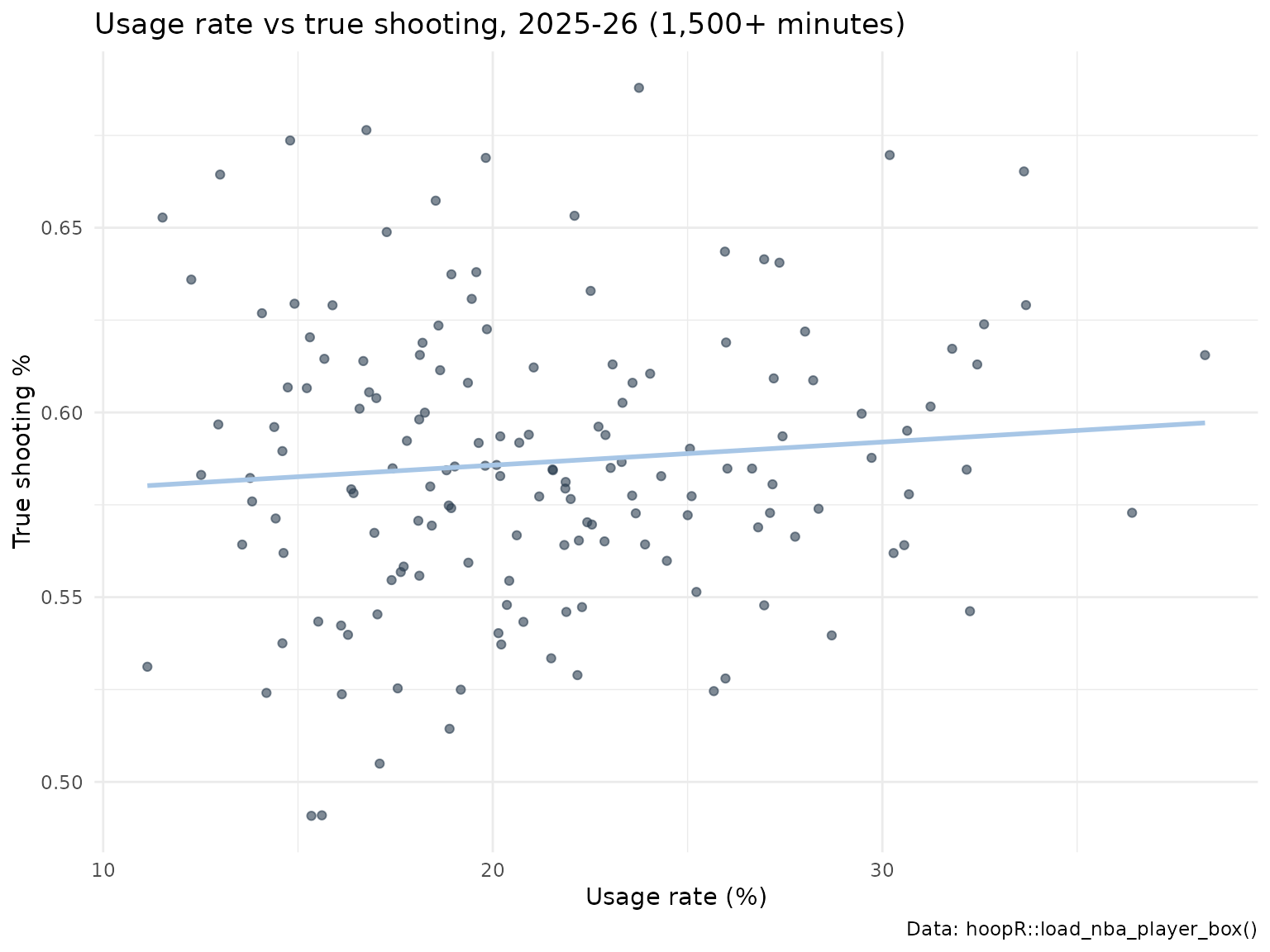

Scatter plot of usage rate against true shooting percentage for NBA players with at least 1,500 minutes in the 2025-26 regular season.

Per-minute and per-possession stats

Counting stats depend on playing time. nba_per_minutes() rescales chosen columns to a per-36-minute basis and nba_per_possessions() to per 100 possessions; both add new {col}_per_{n} columns and leave the originals alone.

players |>
  filter(min >= 1500) |>
  nba_per_minutes(cols = c("pts", "ast", "tov"), minutes = "min", per = 36) |>
  arrange(desc(pts_per_36)) |>
  select(athlete_display_name, min, pts, pts_per_36, ast_per_36, tov_per_36) |>
  mutate(across(ends_with("_36"), \(x) round(x, 1))) |>
  head(5)
#> # A tibble: 5 × 6
#>   athlete_display_name      min   pts pts_per_36 ast_per_36 tov_per_36
#>   <chr>                   <dbl> <int>      <dbl>      <dbl>      <dbl>
#> 1 Shai Gilgeous-Alexander  2262  2117       33.7        7.1        2.4
#> 2 Luka Doncic              2293  2143       33.6        8.3        4  
#> 3 Kawhi Leonard            2087  1813       31.3        4          2.3
#> 4 Victor Wembanyama        1893  1618       30.8        3.8        3  
#> 5 Jaylen Brown             2443  2038       30          5.4        3.8

team_season |>
  left_join(ff |> select(team, tov, oreb), by = "team") |>
  nba_per_possessions(cols = c("pts", "tov", "oreb"), possessions = "poss", per = 100) |>
  select(team, pts_per_100, tov_per_100, oreb_per_100) |>
  mutate(across(-team, \(x) round(x, 1))) |>
  head(5)
#> # A tibble: 5 × 4
#>   team  pts_per_100 tov_per_100 oreb_per_100
#>   <chr>       <dbl>       <dbl>        <dbl>
#> 1 OKC          116         12.3          9.3
#> 2 DET          114.        14.7         12.7
#> 3 SA           117.        13           11.2
#> 4 BOS          117.        12.6         12.8
#> 5 NY           117.        13.6         12.8

pts_per_100 is exactly offensive rating.

Adding several metrics at once

nba_add_advanced_metrics() scans a box score for familiar column names (pts, fgm, fga, fg3m, ftm, fta, oreb, dreb, ast, stl, blk, pf, tov and common aliases) and appends TS%, eFG%, FT rate, TOV%, assist-to-turnover ratio and Hollinger’s Game Score. ESPN’s long names are not among the aliases, so rename first:

player_box |>
  transmute(
    athlete_display_name, game_id, pts = points, fgm = field_goals_made,
    fga = field_goals_attempted, fg3m = three_point_field_goals_made,
    ftm = free_throws_made, fta = free_throws_attempted,
    oreb = offensive_rebounds, dreb = defensive_rebounds, ast = assists,
    stl = steals, blk = blocks, pf = fouls, tov = turnovers
  ) |>
  nba_add_advanced_metrics() |>
  arrange(desc(game_score)) |>
  select(athlete_display_name, pts, ts_pct, efg_pct, game_score) |>
  head(5)
#> # A tibble: 5 × 5
#>   athlete_display_name   pts ts_pct efg_pct game_score
#>   <chr>                <int>  <dbl>   <dbl>      <dbl>
#> 1 Bam Adebayo             83  0.670   0.547       60.5
#> 2 Nikola Jokic            56  0.900   0.810       59.8
#> 3 Nikola Jokic            55  0.915   0.891       53.2
#> 4 Luka Doncic             60  0.782   0.75        51.8
#> 5 Kawhi Leonard           55  0.821   0.75        51.6

Game Score (nba_game_score()) is John Hollinger’s single-game rating, scaled like points: PTS + 0.4 FGM - 0.7 FGA - 0.4 (FTA - FTM) + 0.7 OREB + 0.3 DREB + STL + 0.7 AST + 0.7 BLK - 0.4 PF - TOV.

The same metrics for men’s college basketball

The helpers are league-agnostic. College games are 40 minutes (two 20-minute halves, five-minute overtimes), so quote pace per 40 minutes: 40 * possessions / (minutes / 5). The ESPN college player box records whole minutes, so we round each team’s summed minutes to the nearest regulation-plus-overtime total.

mbb_team <- load_mbb_team_box(seasons = season) |>
  filter(season_type == 2) |>
  transmute(game_id, team_id, team = team_display_name, opp_id = opponent_team_id,
            pts = team_score, fga = field_goals_attempted, fta = free_throws_attempted,
            oreb = offensive_rebounds, tov = total_turnovers)

mbb_minutes <- load_mbb_player_box(seasons = season) |>
  filter(season_type == 2) |>
  group_by(game_id, team_id) |>
  summarise(min = sum(minutes, na.rm = TRUE), .groups = "drop") |>
  mutate(team_min = 200 + 25 * pmax(round((min - 200) / 25), 0))

mbb_games <- mbb_team |>
  inner_join(mbb_team |> select(game_id, opp_id = team_id, opp_pts = pts, opp_fga = fga,
                                opp_fta = fta, opp_oreb = oreb, opp_tov = tov),
             by = c("game_id", "opp_id")) |>
  inner_join(mbb_minutes, by = c("game_id", "team_id")) |>
  mutate(poss = (nba_possessions(fga, fta, oreb, tov) +
                   nba_possessions(opp_fga, opp_fta, opp_oreb, opp_tov)) / 2)

mbb_season <- mbb_games |>
  group_by(team_id, team) |>
  summarise(gp = n(), pts = sum(pts), opp_pts = sum(opp_pts), poss = sum(poss),
            team_min = sum(team_min), .groups = "drop") |>
  filter(gp >= 20) |>
  mutate(
    tempo = 40 * poss / (team_min / 5),
    ortg = nba_offensive_rating(pts, poss),
    drtg = nba_defensive_rating(opp_pts, poss),
    net = nba_net_rating(ortg, drtg)
  )

mbb_season |>
  arrange(desc(net)) |>
  select(team, gp, tempo, ortg, drtg, net) |>
  mutate(across(tempo:net, \(x) round(x, 1))) |>
  head(10)
#> # A tibble: 10 × 6
#>    team                        gp tempo  ortg  drtg   net
#>    <chr>                    <int> <dbl> <dbl> <dbl> <dbl>
#>  1 Duke Blue Devils            34  66.5  124.  95    28.8
#>  2 High Point Panthers         34  70.9  126.  98.3  27.6
#>  3 Gonzaga Bulldogs            33  69.7  122.  94.3  27.3
#>  4 Saint Louis Billikens       33  71.3  122.  97.5  24.9
#>  5 Michigan Wolverines         34  70.7  122.  97.6  24.8
#>  6 Iowa State Cyclones         34  67.6  121.  96.4  24.6
#>  7 Arizona Wildcats            34  70.6  122.  97.1  24.5
#>  8 Houston Cougars             34  64.3  120.  97.5  22.2
#>  9 Illinois Fighting Illini    32  65.6  127. 105.   21.8
#> 10 Miami (OH) RedHawks         32  71.4  125. 104.   21.3

These are raw ratings: they do not know who a team played. A mid-major that beats weak opponents by 20 looks as good as a power-conference team that beats strong ones by 20. Opponent-adjusted ratings fix that; the SportsDataverse publishes them as load_mbb_ratings(), and the team ratings model article explains how they are built. Our raw numbers should line up with that file’s unadjusted raw_o / raw_d columns:

ratings <- load_mbb_ratings(seasons = season)

if (nrow(ratings) > 0) {
  check <- mbb_season |>
    mutate(team_id = as.character(team_id)) |>
    inner_join(ratings |> mutate(team_id = as.character(team_id)) |>
                 select(team_id, raw_o, raw_d, adj_em),
               by = "team_id")
  c(
    teams = nrow(check),
    cor_ortg_raw_o = round(cor(check$ortg, check$raw_o), 3),
    cor_drtg_raw_d = round(cor(check$drtg, check$raw_d), 3),
    cor_net_adj_em = round(cor(check$net, check$adj_em), 3)
  )
}
#>          teams cor_ortg_raw_o cor_drtg_raw_d cor_net_adj_em 
#>        365.000          0.998          0.997          0.785

The ratings file reads a parquet asset, so it needs the arrow package; without it the loader returns an empty table and the check is skipped.

Where to go next

Put efficiency on the court: shot charts and court plots.
From team efficiency to player impact: the NBA player impact model and the college RAPM model, which credit each player for possession outcomes while controlling for teammates and opponents.
Opponent adjustment: the college team ratings model.
Recipes for common questions: the NBA cookbook and men’s college basketball cookbook.
Live, single-game box scores: the ESPN endpoints article.
Every helper: Basketball Analytics Utilities in the reference.

Saiem Gilani